
Chance as Design Element
Chance as Design Element
About the importance of maths for successful game design.
Introduction
Game designers sometimes tend to neglect the scientific aspects of their field, maths and it's significant importance for successful game design especially. (Freyermuth 2015) Taking a look at the most popular game development websites seems to confirm this, as you are hard pressed to find even a single article about maths on the front page. This essay wants to increase awareness about why a deeper understanding of mathematic principles is absolutely necessary if you strive to be the best game designer you can be.
Chance and Game Experience
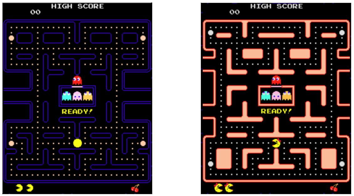
Putting Namco's Pac-Man (left) and Midway's Ms. Pac-Man (right) side by side creates the impression, that the games are identical. You move through a maze collecting points while trying to dodge ghosts that kill you. (Pittman 2017)
You are forgiven to think that. The massive difference only shows itself when searching the internet for strategy guides or when watching the world championships of those games: Pac-Man players are asked to learn movement patterns by heart, which, when executed correctly, will guarantee a win. (Pittman 2017) Therefore, the challenge lies in the correct memorization of many patterns and the development of the hand eye coordination needed to execute them. Players of Ms. Pac-Man, however, are asked to play strategically and react to the position of the ghosts.
This severe difference in game experiences can be traced back to the behaviour of the ghosts. While their pathfinding is strictly deterministic in Pac-Man, in Ms. Pac-Man it contains randomized variables. This turns memorizing predetermined movement patterns useless. This has been confirmed by PacManPlus, an Atari 7800 & NES Developer at Midway:
„[…] the main difference in the Monster AI between Pac-Man and Ms. Pac-Man, is that in Ms. PacMan, Blinky and Pinky randomly move about the maze while in the first 7 seconds instead of going into their corners. This was probably done to make patterns almost impossible […]“ (PacManPlus 2005)
"To a certain extent, games should be unpredictable" (Adams and Dormans 2012) and chance - together with human choice and complex mechanics - is one of three things that can introduce unpredictability into your game.


For tree charts for all nds (n: number of dice, s: number of sides) we derive that a targeted step has a probability of p = 1/s. The probability to land on a certain end of the chart is p = (1/s)ⁿ.
This, however, does not explain why the probability distribution of our 2d6 isn't linear. The reason is, that our tree chart knows the difference between heads + tails and tails + heads; a rolled value of 3, however, does not distinguish between 1+2 and 2+1.

If we assign the values 0 and 1 to heads and tails and take the sum on our way down through the chart (like we'd add up the values of two dice), we'll see that the probability to get the final value of 1 is twice as high as getting 0 or 2, because there are twice as many ends with a 1 compared to the others. This means, we have to multiply the chance to get a certain final value with the number of ends with that value. The number of ends represents the number of different combinations k with said value as a result:
p(value) = k(1/s)ⁿ
Now this probability distribution looks a lot closer to what we had with our 2d6. Now we can explain why: A 7, for example, can be rolled with the six combinations 1+6, 2+5, 3+4, 4+3, 5+2 and 6+1, but a 12 can only be rolled with one: 6+6. This yields the following probabilities:
p(7) = k(1/s)ⁿ = 6(1/6)² = 1/6
p(12) = k(1/s)ⁿ = 1(1/6)² = 1/36
We can now say, that the right choice between a d12 or 2d6 depends on the game experience we want to create. If we want more dice rolls to be near average, we choose 2d6. If we want every value to occur evenly, we choose d12.

Chance and it's Nature
Let's imagine we'd be creating a board game with chance as an element. We can choose between a plethora of different dice and card sets. To choose the correct one and to be able implement it in favor of the wanted game experience, we need to understand it's nature (and that of chance itself); only then are we able to bend that system to our will. (Schreiber 2010)
The tools to do that are found in probability theory, a field of maths. It's based on facts and rules, and probabilites can be calculated exactly. As a game designer you should avoid the mistake of presuming that probability theory lacks accuracy. (Sigman 2006)
Random events are either dependent on each other or not. It's the categorical, distinctive feature splitting the two types of chance. Knowing, which category our system finds itself in is absolutely essential to calculating our probabilities correctly.
Independent Chance
A random event is independent, if it's probability does not depend on the outcome of any other random event. Prime example would be rolling the dice twice: The rolls are completely independent of each other, as the first roll has no influence on the second and vice versa.
Notation
A die with six sides is called a d6. The d stands for dice, the 6 for the number of sides. If theres a number in front of the d, it symbolizes the number of dice, e.g. 2d6 are two dice with 6 sides. It doesn't have to be dice, however, any independent random event with an even distribution of probability will work: e.g. a coin is a d2.
Expected Value
Let's say we decide to use a regular d6 for our board game. Dice have that special property that every side of theirs has an equal probability to get rolled. This gives us the ability to calculate their expected value E by taking the sum of all sides' values and dividing it by the number of sides. The expected value for our d6 with the six sides of 1,2,3,4,5 and 6 would therefore be:
E(d6) = (1+2+3+4+5+6)/6 = 3.5
We can now design and balance our board around the fact that the average value rolled will be 3.5. (Schreiber 2010)
Probability Distributions
Now, let's say we deem 6 to be way too small of a maximum roll, we want to increase it to 12. We now have two sensible choices: We can double the number of dice (turning our d6 into a 2d6) or the number of sides (turning it into a d12).
These choices are not equivalent. This shows when we take a look at their probability distributions. The x-axis shows possible rolls, the y-axis their probability, our d12 is blue and our 2d6 is orange.

D12's probability distribution is linear. However, 2d6's median values have a higher probability compared to it's extremes. This is due to 2d6 not describing one random event, but two. Let's delve a little deeper into probability theory to understand this. (Flick 2017)
Conditional Probability
One of the most important skills to have while dealing with systems of chance is the ability to calculate probabilities of conditional random events: events, that require the occurrence of other events. (Sigman 2006)

These can be visualized using a tree chart. We're seeing two flips of a coin, a 2d2. We start right at the top: No coin has been flipped yet and we can go one of two paths, heads or tails. Flipping a coin chooses one path at random. This means, every path has a 50% chance of being taken. This continues until we reach the lower end of the tree chart. (Sigman 2006)
With this knowledge we can declare that the probability to get tails is p = 1/2 and the probability to get tails twice in a row is p*p = 1/2 * 1/2 = 1/4.
This, however, does not explain why the probability distribution of our 2d6 isn't linear. The reason is, that our tree chart knows the difference between heads + tails and tails + heads; a rolled value of 3, however, does not distinguish between 1+2 and 2+1.

If we assign the values 0 and 1 to heads and tails and take the sum on our way down through the chart (like we'd add up the values of two dice), we'll see that the probability to get the final value of 1 is twice as high as getting 0 or 2, because there are twice as many ends with a 1 compared to the others. This means, we have to multiply the chance to get a certain final value with the number of ends with that value. The number of ends represents the number of different combinations k with said value as a result:
p(value) = k(1/s)ⁿ
Now this probability distribution looks a lot closer to what we had with our 2d6. Now we can explain why: A 7, for example, can be rolled with the six combinations 1+6, 2+5, 3+4, 4+3, 5+2 and 6+1, but a 12 can only be rolled with one: 6+6. This yields the following probabilities:
p(7) = k(1/s)ⁿ = 6(1/6)² = 1/6
p(12) = k(1/s)ⁿ = 1(1/6)² = 1/36
We can now say, that the right choice between a d12 or 2d6 depends on the game experience we want to create. If we want more dice rolls to be near average, we choose 2d6. If we want every value to occur evenly, we choose d12.
Further Conclusions

This knowledge allows us to draw even further conclusions. If we take a look at this graph we can see, that this effect of compression towards the average increases in tandem with the number of events increasing.
This means, the more often a random event occurs, the higher the probability of it's sum being around the average; Which means, the more often different parties repeat said random event, the smaller the expected difference between their own sums.
For our board game, this would mean: Increasing the number of dice rolls in a match will decrease the impact isolated streaks of good or bad luck have on the final outcome. That's something to keep in mind, for sure.
Bernoulli Experiments
We're not only able to calculate the probability of dice rolls, we can also calculate that of a specific outcome occurring for a set amount of times. Requirements for this are that the probability distribution of the random event is linear and that event and counter event are defined in such a way that the sum of their probabilities is 1. This means, that if the event has a 30% chance of happening, it's counter event (the event not happening) needs to have a chance of 70% for all possibilities to be covered. Emperiments of this sort are called Bernoulli experiments.
Let's get back to our mental board game. Our game designer wants to indroduce a dice check event, a gatekeeper that can only be defeated by rolling at least two 6s with three rolls of 2d6. What's the probability of that gatekeeper being defeated? Try to estimate the result before moving on, let's see how good your mathematical intuition is!
First, we need to determine if this really is a Bernoulli experiment. For it to be one, we need to be able to answer each and every of the following questions with "yes".
Is there a set amount of repeats n?
Yes, the amount of repeats n is 3.
Are the random events independent?
Yes, the events are rolls of 2d6, which are independent.
Do the events have a linear probability distributions?
Actually, no. The probability distribution of 2d6 is not linear, as shown above. A 2d6 can be split into two rolls of d6, however, whose probability distribution is linear. The number of repeats corrects itself to n = 3 * 2 = 6.
Are all possibilities covered?
We have to define event and counter event. The event is 'Rolling a 6' with p(event) = 1/6, the counter event would be 'Not rolling a 6' with p(counter) = 5/6. The sum of their probabilities is p(event) + p(counter) = 1/6 + 5/6 = 1. Yes, all possibilities are covered.
Are we asking for the event to occur a set amount of times x?
Yes, we're asking for the event to occur twice: x = 2.
We've answered all the questions positively, which means we do have a Bernoulli experiment on our hands: We want to calculate the probability of rolling a 6 twice with 6 rolls of a d6.
The first combination we want to deal with is rolling a 6 on the first two rolls, then not rolling any with the other four. Like earlier, we just multiply the probabilities of each individual event to get the result.
p = (1/6)^2 * (5/6)^4 = 0.0130 = 13%
Now we multiply p with the number of possible permutations k (first and second, first and third, etc). Luckily, we don't need to calculate k by hand. Another field of math, combinatorics, has exactly what we need: the binomial coefficient k = n choose x.
p(2) = (6 choose 2) * 0.013 = 0.0201 = 20.1%
This is the probability p(2) of rolling exactly two 6s with 6 rolls of d6. Not quite what we need, though. We asked for the probability p(≥2) of rolling at least two. To get this, we need to caclulate and add the probabilities p(3), p(4), p(5) and p(6).
p(≥2) = p(2) + p(3) + p(4) + p(5) + p(6) = 26.4%
The probability of defeating the gatekeeper is 26.4%. Is this close to what you estimated?
This means around 3 of 4 dice checks would fail. That's knowledge that truly helps us balance our game.
Negation
Calculating this probability was pretty time consuming. Sometimes, it's easier to calculate the probability of something not happening, then subtracting the result from 1.
p(≥2) = 1 - p(<2) = 1 - (p(0) + p(1)) = 1 - (0.334 + 0.402) = 100% - 73.6% = 26.4%
No Guarantees
We're multiplying probabilities of certain events to calculate the probabilities of combinations and 1 ≥ p ≥ 0. This means that nothing will ever have a guarantee of happening, except when p is 1 or 0. To create a guarantee, we'd have to remove chance completely.
Let's say we want to introduce a door into our board game. The board sports 3 consumable switches, each with a chance to open the door. We want to create the game experience, that the player doesn't know which switch is correct. If we implemented a system of independent random events here, we either have to increase the chance of a switch to open a door to 100% (which defeats the purpose) or live with the fact that there's a certain percentage of games where the door just won't open (which would break the game).
Optimal would be a mix between them: One of the switches is guaranteed to open the door, but which one is determined by chance. Luckily, theres still this second type of chance we didn't talk about yet.
Dependent Chance
As the name suggests, dependent chance describes random events dependent on each other. Results of previous events do have an influence on events in the future. The prime example for systems of that sort are decks of cards. (Schreiber 2010)
Let's look at a deck with n = 6 cards numbered from 1 to 6. If you draw a card, the chance to draw a 6 is 1/6. If you don't draw one, the chance for the next card to be a 6 is 1/5 as there will be less cards in the deck. The chance to draw a 6 keeps increasing until it reaches 100% on the last card or until a 6 is drawn. When a 6 is drawn it drops to 0% as there is no 6 left in the deck. This gives us the guarantee that exactly one 6 will be drawn. (Schreiber 2010)
This guarantee holds for every card in the deck, which means we can calculate the sum of all drawn values after drawing the entire deck:
E(total) = 1+2+3+4+5+6 = 21.
This isn't rocket science but very relevant for our game design. If a player draws a high value card, not only does he gain the benefit of that high value, the other players also lose out on ever being able to draw that high value themselves. This makes "catching up" to a player who got lucky on the first draws less likely compared to rolls of dice, which don't have that effect. (Schreiber 2010)
These peculiarities of dependent and independent chance can have a serious impact on our game experience. Choosing the right type for the right situation is of utmost importance. For our three switches, dependent chance is what we should be going for. For game events independent of each other we should use independent chance.
Conditional Probability
Calculating conditional probabilities works just like with independent random events. We multiply the probabilities of each event with each other. The main difference is that p changes with every event. This means we have to do our calculations step by step, too. We calculate recursively.
Let's go back to our deck of 6 cards. We now want to calculate the probability p(4), drawing the 6 with the fourth card. The necessary events that need to happen are the following:
- The first card is not a 6, p = 5/6
- The second card is not a 6, p = 4/5
- The third card is not a 6, p = 3/4
- The fourth card is a 6, p = 1/3
p(4) = (5/6)*(4/5)*(3/4)*(1/3) = 1/6
Surprise, surprise! The chance for the 6 to be at a specific position in a deck of 6 cards is 1/6. This is the same for every position p(x), which means the probability distribution is linear again. For our three switches this would mean, that the chance to be the correct switch is evenly distributed between all switches - which is exactly what we want.
What makes this even easier for us is that we don't have to consider the number of permutations k because we're calculating step by step, anyway. The order of events is predetermined, thus k is always 1.
Don't be fooled, though. While understanding how to calculate probabilities like this is more intuitive than independent chance, calculating probabilities of larger systems of chance can get extremely time consuming. (Schreiber 2010)
Conclusion
Games do need to be unpredictable to a certain extent. If you can predetermine the outcome of a game with absolute certainty, there would be no reason to play it. Chance is one of three tools in a game designer's toolkit which are able to infuse your game with such unpredictability. (Adams and Dormans 2012)
Although, to create art using a tool - and game design is an art (Schell 2016) - you need to master it. To master even the most basic systems of chance, dice and cards, a general understanding of probability theory is absolutely necessary. Without maths, there is no safe handling of chance and you lose access to one of the most important tools of your kit.
Sources
Adams, Ernest; Dormans, Joris (2012): Game Mechanics. Advanced Game Design.
Flick, Jasper (2017): Anydice.com. Probability Calculator. Online verfügbar unter http://anydice.com/.
Freyermuth, Gundolf S. (2015): Games | Game Design | Game Studies. Eine Einführung.
PacManPlus (2005): Pac-Man ghost AI question. Hg. v. atariage.com. Online verfügbar unter http://atariage.com/forums/topic/68707-pac-man-ghost-aiquestion/?hl=%20pacman%20%20dossier, zuletzt geprüft am 26.11.2017.
Pittman, Jamey (2017): The Pac-Man Dossier. Online verfügbar unter https://www.gamasutra.com/view/feature/3938/the_pacman_dossier.php?print=1, zuletzt geprüft am 24.12.2017.
Schäfer, Frederik (2012): http://www.poissonverteilung.de/binomialverteilung.html, zuletzt geprüft am 11.12.2017.
Schell, Jesse (2016): Die Kunst des Game Designs. Bessere Games konzipieren und entwickeln. Unter Mitarbeit von Maren Feilen. 2. Auflage. Frechen: mitp (Safari Tech Books Online).
Schreiber, Ian (2010): Game Balance Concepts. Level 4: Probability and Randomness. Online verfügbar unter https://gamebalanceconcepts.wordpress.com/2010/07/28/level-4-probability-andrandomness/.
Sigman, Tyler (2006): Statistically Speaking, It's Probably a Good Game, Part 1: Probability for Game Designers. Hg. v. Gamasutra. Online verfügbar unter https://www.gamasutra.com/view/feature/130218/statistically_speaking_its_.php page=3.
StrategyWiki (2017): Ms. Pac-Man/Walkthrough, zuletzt aktualisiert am 11.02.2017, zuletzt geprüft am 24.12.2017.
Comments
Post a Comment